Tracing the Transformer: How Self-Attention Actually Works

Every large language model you’ve used — GPT, Claude, Llama, BERT before them — is built out of the same core mechanism, repeated dozens of times: the Transformer block. It’s easy to wave your hands and say “it’s attention,” but the actual mechanics are simple enough to trace end to end. This post does that: from a sequence of tokens to a single self-attention head, to a full block, to a stack of them.

From words to vectors

A Transformer never sees words. It sees vectors. The first thing that happens to an input sequence is:

1. Tokenization — the text is split into subword pieces, each mapped to an integer id.
2. Embedding — each id is looked up in an embedding table, producing a vector (typically a few hundred to a few thousand dimensions).
3. Positional encoding — because the rest of the network has no built-in sense of order (unlike an RNN, which processes tokens one at a time), a position-dependent vector is added to each token embedding so the model can tell “the cat sat” from “sat the cat.”

The result is a matrix $X$ of shape (sequence length, model dimension) — one row per token. Everything from here on is matrix arithmetic over $X$.

The core idea: attention as a lookup

Self-attention lets every token look at every other token and decide how much to weight each one when building its own updated representation. The mechanism is a soft, differentiable key-value lookup:

• Query ($Q$) — “what is this token looking for?”
• Key ($K$) — “what does this token contain, as a label to be matched against?”
• Value ($V$) — “what does this token actually offer, once it’s been picked?”

$Q$, $K$, and $V$ are all linear projections of the same input $X$ (using three separate learned weight matrices), which is why this is called self-attention — the sequence is attending to itself.

The similarity between every query and every key is computed with a dot product, scaled down, turned into a probability distribution with softmax, and used to take a weighted sum of the values:

\[\text{Attention}(Q, K, V) = \text{softmax}\left(\frac{QK^{\top}}{\sqrt{d_k}}\right)V\]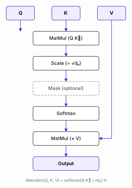

Scaled dot-product attention — the operation repeated inside every head.

Two details are easy to miss but matter a lot in practice:

• The scale factor, $\sqrt{d_k}$. Dot products grow with dimensionality. Without scaling them down, large values push softmax into a regime where its gradient is nearly zero almost everywhere, and training stalls.
• The optional mask. In a decoder, a token must not attend to positions that come after it — otherwise the model could “cheat” by looking at the answer it’s supposed to predict. The mask sets those positions to $-\infty$ before the softmax, so they get a weight of zero.

Multi-head attention: many lookups at once

A single attention operation gives the model one notion of “relevance.” In practice, different tokens need to relate to each other in different ways at once — syntax, coreference, position, topic. Multi-head attention runs several smaller attention operations in parallel, each with its own learned $Q$, $K$, $V$ projections into a lower-dimensional subspace, then concatenates the results and projects them back:

\[\text{MultiHead}(Q,K,V) = \text{Concat}(\text{head}_1, \dots, \text{head}_h)W^O, \quad \text{head}_i = \text{Attention}(QW_i^Q, KW_i^K, VW_i^V)\]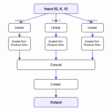

Multi-head attention — h attention operations run in parallel subspaces, then combined.

Splitting into heads costs nothing in total compute — each head just works on a slice of the model dimension — but gives the model several independent “attention patterns” to learn instead of one.

Assembling a block

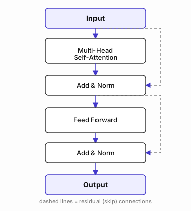
Multi-head attention alone is just a weighted average — stacked on its own, it wouldn’t be able to represent much. Two more ingredients turn it into something that can be trained dozens of layers deep:

• Residual connections. The input to a sub-layer is added back to its output (x + Sublayer(x)) rather than being replaced by it. This gives gradients a direct path back through the network, which is what makes it practical to stack many blocks without training collapsing.
• Layer normalization. Applied after each residual sum, it rescales activations to keep training stable as depth increases.
• A position-wise feed-forward network. After attention mixes information across token positions, a small two-layer MLP (applied identically and independently to each position) gives the model capacity to transform within a position.

One encoder block: attention and a feed-forward network, each wrapped in a residual connection and layer norm.

Stacking blocks: encoders, decoders, and masking

A full Transformer is a stack of these blocks — the original architecture used six of each. The encoder and decoder differ in one key way:

• Encoder blocks use unmasked self-attention: every token can attend to every other token, in both directions. This is the right setup for building a representation of a complete input, like a sentence to be translated or classified.
• Decoder blocks use masked (causal) self-attention — the mask from the diagram above — so that token $i$ can only attend to tokens $1 \ldots i$. This is what lets the same architecture be trained to predict the next token and then generate text one token at a time at inference. Decoder-only models like GPT are, essentially, a stack of nothing but this kind of block.

Everything downstream of this — larger models, longer context windows, better positional schemes — builds on exactly this stack. There’s no hidden mechanism beyond it; it’s matrix multiplications, a softmax, and a great deal of scale.

Further reading: the original paper, Attention Is All You Need (Vaswani et al., 2017), and Jay Alammar’s The Illustrated Transformer, which walks through the same mechanics with more visuals than fit in one post.